Introduction
This project was a presentation I had on Causal Inference. Specifically, I did a summary of the RDD and Weighting Design methods.
Overview of Methods
- Regression Discontinuity Design (RDD):
- Sharp nonparametric regression discontinuity.
- Before-After (BA) Design:
- Interrupted time-series for estimating treatment effects.
- Treatment Effect Estimation with Weighting:
- Addresses covariate imbalance using propensity scores.
Regression Discontinuity Design (RDD)
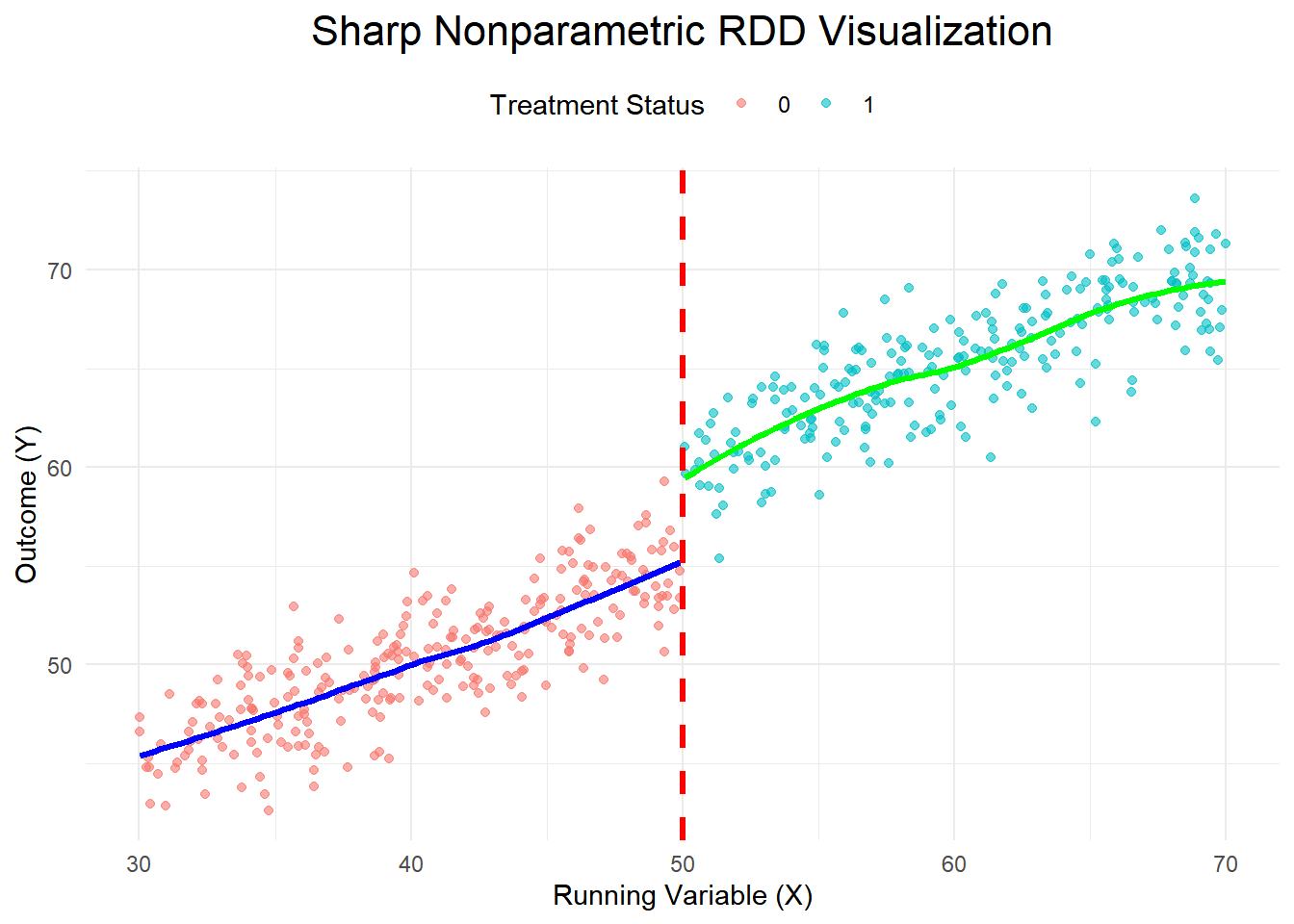
Sharp Nonparametric RDD
Setup:
- Treatment determined by a threshold \(\tau\) on the running variable variable \(x\).
- Example: Eligibility for aid based on income \(d = 1[x \geq \tau]\).
Model:
\[
y = \beta_d d + g(x) + u
\]
- \(\beta_d\): Treatment effect.
- \(g(x)\): Smooth function of \(x\).
Key Assumptions:
- Continuity in Observables: \(g(x)\) is continuous at \(x = \tau\).
- Continuity in Unobservables: \(E(u|x)\) is the same just above and below \(\tau\).
Estimation:
\[
\beta_d = \lim_{x \to \tau^+} E(y|x) - \lim_{x \to \tau^-} E(y|x)
\]
Illustration
Simulating Data and Visualization of Concept
Code
# Load necessary libraries
library(ggplot2)

# Step 1: Simulate Sharp RDD Data
set.seed(123)
n <- 500
threshold <- 50

# Generate data
x <- runif(n, 30, 70)  # Running variable
treatment <- as.numeric(x >= threshold)  # Treatment assignment
y <- ifelse(
  treatment == 1,
  30 + 0.5 * x + 5 + rnorm(n, mean = 0, sd = 2),  # Treated outcome
  30 + 0.5 * x + rnorm(n, mean = 0, sd = 2)       # Control outcome
)

# Create a data frame
data <- data.frame(X = x, Treatment = treatment, Outcome = y)

# Step 2: Create the Scatter Plot with Regression Lines
ggplot(data, aes(x = X, y = Outcome, color = factor(Treatment))) +
  geom_point(alpha = 0.6) +  # Scatter points
  geom_smooth(data = subset(data, Treatment == 0),
              method = "loess", se = FALSE, color = "blue", size = 1.2) +
  geom_smooth(data = subset(data, Treatment == 1),
              method = "loess", se = FALSE, color = "green", size = 1.2) +
  geom_vline(xintercept = threshold, linetype = "dashed", color = "red", size = 1.2) +
  labs(
    title = "Sharp Nonparametric RDD Visualization",
    x = "Running Variable (X)",
    y = "Outcome (Y)",
    color = "Treatment Status"
  ) +
  theme_minimal() +
  theme(
    plot.title = element_text(hjust = 0.5, size = 16),
    legend.position = "top"
  )
Model Fitting - In a nutshell!
Code
# Load necessary libraries
library(rdrobust)

fit = rdrobust::rdrobust(y = data$Outcome, x = data$X, c = threshold, all = T)

summary(fit)
Sharp RD estimates using local polynomial regression.

Number of Obs.                  500
BW type                       mserd
Kernel                   Triangular
VCE method                       NN

Number of Obs.                  265          235
Eff. Number of Obs.              71           52
Order est. (p)                    1            1
Order bias  (q)                   2            2
BW est. (h)                   5.085        5.085
BW bias (b)                   8.424        8.424
rho (h/b)                     0.604        0.604
Unique Obs.                     265          235

=======================================================================================
        Method     Coef. Std. Err.         z     P>|z|      [ 95% C.I. ]
=======================================================================================
  Conventional     4.813     0.682     7.057     0.000     [3.476 , 6.150]
Bias-Corrected     5.044     0.682     7.396     0.000     [3.707 , 6.380]
        Robust     5.044     0.799     6.316     0.000     [3.479 , 6.609]
=======================================================================================
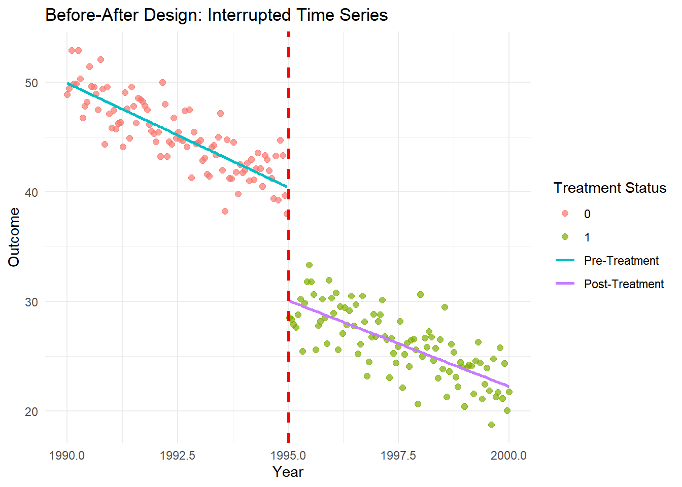
Before-After (BA) Design
Overview
- Concept: Compare outcomes before and after a treatment.
- Example: Assessing the effect of a speed limit law on accident rates.
Model:
\[
y_t = \beta_d d_t + g(t) + u_t
\]
- \(\beta_d\): Treatment effect.
- \(g(t)\): Time trend.
Key Assumptions:
- Treatment effect occurs immediately after intervention.
- Other time-varying factors are minimal near the intervention.
Challenges of BA Design
- Simultaneous Changes: Other factors (e.g., economic trends) may confound results.
- Gradual Effects: Treatment effects that develop slowly are hard to detect.
- No Contemporary Control Group: Relies solely on pre-treatment data as the control.
Illustration
Simulating Data and Visualization of Concept
Code
# Load necessary libraries
library(ggplot2)
library(dplyr)

# Step 1: Simulate Before-After Dataset
set.seed(123)
n <- 200  # Number of observations
break_year <- 1995  # Year of intervention

# Generate data
year <- seq(1990, 2000, length.out = n)
pre_treatment <- year < break_year
treatment <- as.numeric(year >= break_year)

# Simulate outcomes
outcome <- ifelse(
  pre_treatment,
  50 - 2 * (year - 1990) + rnorm(n, mean = 0, sd = 2),  # Pre-treatment trend
  30 - 1.5 * (year - break_year) + rnorm(n, mean = 0, sd = 2)  # Post-treatment trend
)

# Create a data frame
data <- data.frame(Year = year, Treatment = treatment, Outcome = outcome)

# Step 2: Fit Separate Regression Models
pre_model <- lm(Outcome ~ Year, data = data[data$Treatment == 0, ])
post_model <- lm(Outcome ~ Year, data = data[data$Treatment == 1, ])

# Step 3: Visualize the Before-After Trend
ggplot(data, aes(x = Year, y = Outcome)) +
  geom_point(aes(color = factor(Treatment)), size = 2, alpha = 0.7) +
  geom_smooth(method = "lm", data = data[data$Treatment == 0, ],
              aes(color = "Pre-Treatment"), se = FALSE) +
  geom_smooth(method = "lm", data = data[data$Treatment == 1, ],
              aes(color = "Post-Treatment"), se = FALSE) +
  geom_vline(xintercept = break_year, linetype = "dashed", color = "red", size = 1) +
  labs(title = "Before-After Design: Interrupted Time Series",
       x = "Year", y = "Outcome",
       color = "Treatment Status") +
  theme_minimal()
Treatment Effect Estimation with Weighting
Motivation for Weighting
- Observational studies often suffer from selection bias.
- Treated and untreated groups may differ in observed covariates (“x”).
- Weighting adjusts for differences in covariates to estimate:
- Effect on the untreated
- Effect on the treated
- Effect on the population
Basic Idea
Weighting Definition
- Derive weights using the propensity score: \(\pi(x) = P(d = 1|x)\)
- Weights:
- Treated: \(\frac{1}{\pi(x)}\)
- Untreated: \(\frac{1}{1 - \pi(x)}\)
Objective:
- Balance the covariate distributions of treated and untreated groups.
Estimating Treatment Effects
Effect on the Untreated
Treatment Effect:
\[
E(y_1|d = 0) - E(y|d = 0)
\]
Effect on the Treated
Treatment Effect:
\[
E(y|d = 1) - E(y_0|d = 1)
\]
Benefits of Weighting
- Balances covariates between treated and untreated groups.
- Avoids dimension problems associated with regression.
- Improves efficiency of estimators.
Challenges of Weighting
- Small Propensity Scores:
- When \(\pi(x)\) is near 0 or 1, weights can become unstable.
- Model Dependence:
- Relies on correctly specifying \(\pi(x)\).
- Unobserved Confounders:
- Cannot address bias from unobserved factors.
Practical Implementation
- Estimate propensity scores (e.g., logistic regression).
- Compute weights:
- Treated: \(\frac{1}{\pi(x)}\)
- Untreated: \(\frac{1}{1 - \pi(x)}\)
- Estimate treatment effects using weighted averages or regression.
Back to top